CLIWOC (British, Spanish and Dutch shipping 1750-1855): Getting the data into R

on the Spatial analysis blog a nice visualisation of the major shipping route of the British, Dutch and Spanish fleet in 1750-1850 was presented recently. based on the Climatological Databases for the World's Oceans (CLIWOC). another even nicer visualisation of the same data was presented by  unconsenting. in neither case any code was provided, in particular with regards to just getting the data into a readable format. so i did some digging into the the CLIWOC home-page, with just that particularity in mind.
being a Linux Fedora user i started limiting my, albeit quick trial, with what was supposed to be a linux/unix readable format on the CLWVOC main database release page. this being CLIWOC15.Z file. that trial was not very successful. managed to read in the data into R after getting rid of some "unwanted" characters that R did not "like". however, the fields (columns supposed to be semicolon delimited) was more or less messed up. and the number of records were also less than specified on the page. most importantly the trial was based on non-reproducible code within the R-environment.
so, reluctantly i decided to have a go at the MS Access databases CLIWOC15_2000.zip source, albeit not having high hopes that i could find a solution that would work withing the Linux environment. but after some search on the web on how to read mdb format directly into R environment within Linux i stumbled across this post. In particular: "Use mdb.get() from Hmisc package to import entire tables from the database into dataframes." just what the doctor ordered. now i had the Hmisc library already installed. but I did not have the success with the mdb.get() function. reading the help file on mdb.get (?mdb.get) one "gets": "Uses the mdbtools package executables mdb-tables, mdb-schema, and mdb-export. in Debian/Ubuntu Linux run apt get install mdbtools." being a Fedora user the equivalent command to install the mdbtools is:
yum install mdbtools
with that I was ready to go. with the following  code i managed to achieve my objective of getting the CLIWOC MS Access data into R environment within the Linux framework (as well as do some very crude initial ggplot2):

require(Hmisc) # need also mdbtools, in Fedora do  >yum install mdbtools
path <- "yourworkingdirectory"
URL <-  "http://www.knmi.nl/"
PATH <- "cliwoc/download/"
FILE <- "CLIWOC15_2000.zip"
download.file(paste(URL,PATH,FILE,sep=""),
              paste(path,"CLIWOC15_2000.zip",sep=""))
dir <- unzip(paste(path,"CLIWOC15_2000.zip",sep=""))
file <- substr(dir,3,nchar(dir))
dat <- mdb.get(file)
tmp <- dat$CLIWOC15[,c("Lon3","Lat3")]
require(ggplot2)
ggplot(tmp,aes(Lon3,Lat3)) + geom_point(alpha=0.01,size=1) + coord_map() +
  ylim(-90,90)

Created by Pretty R at inside-R.org

getting ICES 1903-1949 catch statistics into R

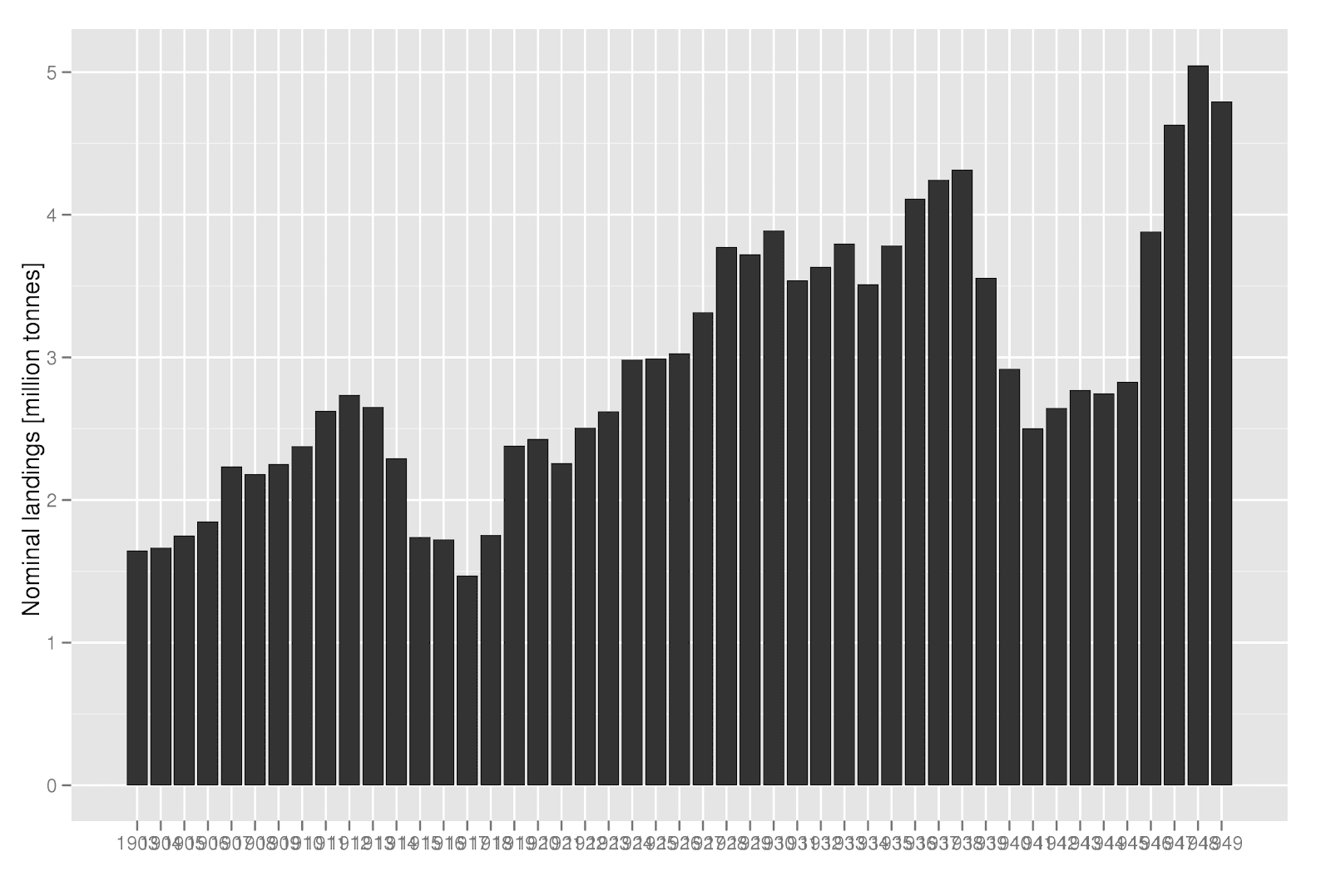
in the last post i showed how to get the nominal north east atlantic landings data from 1950 onwards into a usable format in R. this time around a script that shows how to import zipped excel files from 1903 to 1949 is provided. finalizing with a ggplot of the total reported landings over the period.

again the data is available at the web site (http://www.ices.dk/fish/CATChSTATISTICS.asp) as excel files. the twist is that the files are stored in a zipped format and there are separate excel files for each country. and within each country file there is a separate worksheet for each of the years. within each worksheet the data are again stored in a wide format, the species recorded in the landings is by rows and the area fished is by columns. the number of rows (species recorded) and the number of columns (area fished) differs among different worksheet. and then there are some other nasties here and there in the worksheets, something that took a little trial and error to circumvent in the final script provided.

this is what the final work looked like:
################################################################################
# stuff needed
require(gdata)
require(reshape2)
require(stringr)
require(plyr)

################################################################################
# the source
path <- "YOURDIRECTORY"
URL <-  "http://www.ices.dk/"
PATH <- "fish/statlant/"



################################################################################
# Downloading and extraction of 1903 to 1949 data
FILE <- "ICES1903-49.zip"
download.file(paste(URL,PATH,FILE,sep=""),
              paste(path,"ICES19030-49.zip",sep=""))
dir <- unzip(paste(path,"ICES19030-49.zip",sep=""))

files <- sort(dir[grep("xls",dir)])
files <- substr(files,3,nchar(files))
cntr <- substr(files,1,3)

dat <- NULL
for (i in 1:length(cntr)) {
  print(cntr[i])
for (j in c(2:48)) {
  print(j+1901)
  if (i == 1 & j == 44)  {                     # problem with header character
    tmp <- read.xls(files[i],sheet=j,strip.white=T,stringsAsFactors=F,
                  header=F,skip=1)
    names(tmp) <- c("species","alpha","IVc","IV","VIIa,f","VIId,e","UNK","Total")
  } else {
  tmp <- read.xls(files[i],sheet=j,strip.white=T,stringsAsFactors=F,blank.lines.skip = TRUE)
  }
  if(i == 19 & j == 25) tmp <- tmp[1,1:2]    # Russia 1926 (empty spaces)
  #print(tmp)
  if(ncol(tmp)>1 & nrow(tmp)> 1) {
    rowTotal <- grep("Total",tmp[,1]) # find the location of row Total
    colTotal <- grep("Total",names(tmp)) # find the location of column Total
    if(i == 6  & j == 22) {rowTotal <- 22 ; colTotal <- 8} # France  1923
    if(i == 12 & j == 7)  {rowTotal <- 18 ; colTotal <- 7} # Ireland 1908
    tmp <- tmp[1:(rowTotal-1),1:(colTotal-1)] # exclude anything below and to
                                              #  the right of Total, including the Total
    names(tmp)[1:2] <- c("species","alfa")    # the species acronym column is in most cases left blank
                                        # in some cases it is however names something odd
    tmp <- melt(tmp,id.var=c("species","alfa"))   # turn into long format (kind of like inverse of "Pivot table"
    tmp$variable <- as.character(tmp$variable)
    tmp$value <- str_replace_all(tmp$value,",","")
    tmp$value <- ifelse(tmp$value %in% "-",0,tmp$value)
    tmp$value <- ifelse(tmp$value %in% ".",NA,tmp$value)
    tmp$value <- ifelse(tmp$value %in% "<0.5",0.25,tmp$value)
    tmp$value <- ifelse(tmp$value %in% "",NA,tmp$value)
    tmp$value <- as.numeric(tmp$value)
    tmp$year <- rep(j+1901,nrow(tmp))
    tmp$cUN2 <- cntr[i]
    dat <- rbind(dat,tmp)
  }
} # end loop through sheets (years/worksheet)
} # end loop through countries (xls file)
require(ggplot2)
ggplot(dat,aes(factor(year),weight=value/1e6))+ geom_bar() + xlab("") +
  ylab("Nominal landings [million tonnes]")

the focus here has been on just getting the data into R. more work is needed, in particular when it comes to combining the data from 1903-1949 and 1950-2010. hope i will have some time to work and report on that later.