ICES and NAFO statistical areas viewed in Google Earth

On the ICES Spatial Facility webpage one can obtain a view of the ICES statistical areas. Now since the projection used is more than a bit misleading I was wandering how these statistical areas would look like in Google Earth. Thankfully the shapefiles associated with these rectangles are available to download  from the web page. What follows is less than a bare bone code to convert the shape files into kml files. Except that a bit of a thinning of the spatial codes was needed because the original shapefiles are very detailed for some of the coastal areas resulting in very nonsmoothed zooming etc. in Google Earth. While doing this I also included the NAFO areas. Since I also wanted to see the EEZ on top of this I include a code to convert EEZ shapefiles to kml. The EEZ data were downloaded from the VLIZ Maritime Boundaries Geodatabase.

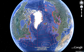
Before running the code below, one needs to download the necessary data onto the local machine and extract the data from the zipped file into a working directory (not needed for NAFO areas - is included in the code below). Once this has been done the following code was used to convert the data into Google Earth format:

setwd("yourWorkingDirectory")
library(maptools)
# gpclibPermit() # may be needed
library(rgdal)
# ices areas
ices_areas = readOGR('ices_areas.shp','ices_areas')
ices_areas <- thinnedSpatialPoly(ices_areas,tolerance=0.04) # takes some time
writeOGR(ices_areas,'ices_areas.kml','ices_areas',driver='KML')
# world eez
eez <- readOGR('World_EEZ_v6_1_simpliefiedcoastlines_20110512.shp',
               'World_EEZ_v6_1_simpliefiedcoastlines_20110512')
writeOGR(eez, "eez.kml", "eez", driver="KML")
# nafo areas
download.file('http://www.nafo.int/about/overview/gis/Divisions.zip',
              destfile='NAFOdivisions.zip')
unzip('NAFOdivisions')
nafo_areas <- readOGR('NAFOdivisions.shp','NAFOdivisions')
writeOGR(nafo_areas,'nafo_areas.kml','nafo_areas',driver='KML')

Created by Pretty R at inside-R.org

Now one only needs to open the  kml files (ices_areas.kml, nafo_area.kml and eez.kml, located in the working directory) in Google Earth. If there are problems with downloading or running the scripts I provide the ices_areas.kml, nafo_areas.kml and eez.kml via my Public Dropbox space (there is also a depth contour in the E-Greenland, Iceland Faero Is. region, see nwwgDepth.kml)
As said, this is very much a bare bone attempt but at least describes the essence of getting a GE view of the ICES and NAFO statistical areas. Zooming in and out is a breeze and by clicking on an area some statistics show up. A snapshot of the broad view as presented in the projection on the ices page vs. the one provided in Google Earth are shown for comparisons. The global EEZ are a bonus :-)